Dispersion GUI mode - the clustered analysis

Before the second analysis with spin clustering will be performed, the relax state will be saved in the file state.bz2 and the program closed. To store the details of the second analysis in a separate log file, relax will be restarted with the command:

$ mpirun -np 8 /data/relax/relax-trunk/relax -multi='mpi4py' -log ∼/tmp/dispersion/log_clustered -gui

When the GUI has started, load the state.bz2 file. If relax is not restarted, all messages will be in a single log file.

For the clustered analysis, we will focus on one group of spins - those from residues :59 to :67. These can be seen to have very similar dynamics:

[basicstyle=\ttfamily \scriptsize,numbers=none]
# Parameter description:  The population for state A.
#
# mol_name  res_num  res_name  spin_num  spin_name  value                 error                   
[snip]
None        59       GLY       None      N             0.991169677577733    0.0254974551085798    
None        60       GLY       None      N          None                  None                    
None        61       GLY       None      N             0.989169345780449  0.000173707304433962    
None        62       GLY       None      N             0.892612114003636     0.156741312688688    
None        63       GLY       None      N             0.991579380015928   0.00101555844987099    
None        64       GLY       None      N             0.983519617639107   0.00141882200997569    
None        65       GLY       None      N             0.993831316342131   0.00840481515172743    
None        66       GLY       None      N             0.996816227018878   0.00495523034494496    
None        67       GLY       None      N             0.987206586948786  0.000217099775069814    
[snip]

[basicstyle=\ttfamily \scriptsize,numbers=none]
# Parameter description:  The exchange rate.
#
# mol_name  res_num  res_name  spin_num  spin_name  value                 error                   
[snip]
None        59       GLY       None      N              1856.39029180567      258.796681611922    
None        60       GLY       None      N          None                  None                    
None        61       GLY       None      N              1706.42820099893      79.5779060629935    
None        62       GLY       None      N              1560.77926730839      246.876174669559    
None        63       GLY       None      N              1448.69535431372      121.940593279104    
None        64       GLY       None      N               1922.2405164604      96.0557804598977    
None        65       GLY       None      N               1333.8423680145      168.000554346898    
None        66       GLY       None      N              1243.45993122534      238.215664971556    
None        67       GLY       None      N              1753.32557147779      78.2028166128168    
[snip]

All other spins will be deselected.

From the non-clustered results, it could be argued that all spins in the entire system experience the same dynamic process, i.e. they have the same p_A and k_ex values. Such an analysis could be performed at a later stage if desired. The dispersion curves for the residue :60 could also be inspected to see that dispersion is likely to be present and another clustered analysis including this spin performed. The number of clustered analyses performed is up to the user - imagination is the only limit.

To start the analysis, open the analysis selection wizard as was performed previously. Name the analysis as `Dispersion - Hansen (clustered :59 to :67)'. Once the analysis is initialised, change the results directory to ∼/tmp/dispersion/clustered. To use the results of the previous analysis to speed up this analysis, as clustering will cause the grid search to be impossibly long, change the “Previous run directory” value to ∼/tmp/dispersion/non_clustered.

Set up the spin systems as for the non-clustered analysis. This time however deselect all spins except for those of residues :59 to :67 (excluding :60). This can be performed by right clicking on the spins in the spin viewer window.

The next step is to cluster these eight spins. In the “Spin cluster IDs” GUI element, click on the “Cluster” button. This launches the relax_disp.cluster user function. Set the cluster ID to “res_59_to_67”, for example, and the spin ID string to “:59-67” (this says all residues from :59 to :67, see section 4.2.2 on page  for details):

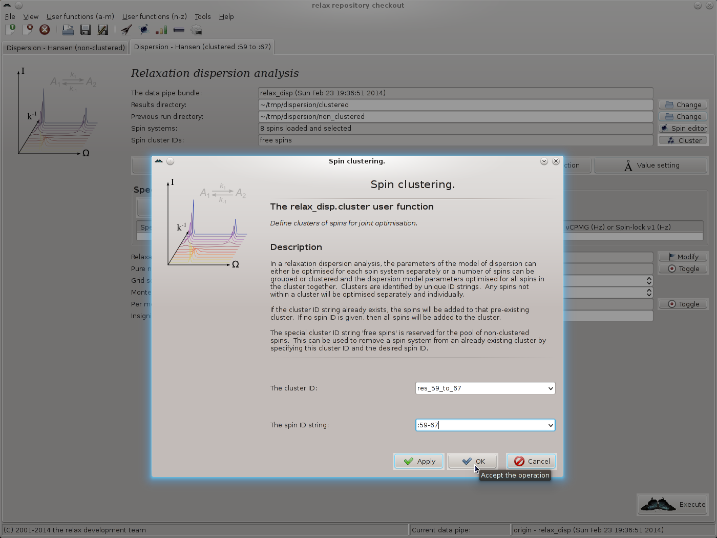
As spin :60 is deselected, that residue will be skipped in the analysis.

Then set the spin isotope and load all of the Sparky peak lists as before. Chose the models `R2eff', `No Rex', `CR72', and `NS CPMG 2-site expanded'. As the `CR72' and `NS CPMG 2-site expanded' were seen as being statistically equivalent in the non-clustered analysis, click on the “Toggle” button of the “Pure numerical solutions” GUI element to avoid the `CR72' model in the model selection step. Actually, as the initial parameters for the `NS CPMG 2-site expanded' model in the dispersion auto-analysis will be taken as the average from the non-clustered analysis, the `CR72' model could be completely skipped.

Ignore the grid search increment setting as this will have no effect. No grid searches will be performed because the results from the non-clustered analysis will be used as the optimisation starting point. Set the Monte Carlo simulations to 200. The main window should now look like:

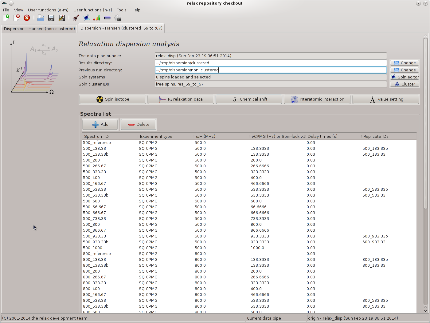
Start the analysis by clicking on the “Execute” button. You should notice that the spin cluster printout in the log messages in the relax controller window now show the text:

[numbers=none]
The spin cluster [':59', ':60', ':61', ':62', ':63', ':64', ':65', ':66', ':67'].

As residue 60 is deselected, it will not be used in the optimisation or any part of the analysis. The full analysis should take a few hours to complete.