The R2eff model

This is the simplest of all models in that the dispersion component of the base data - the peak intensity values - is not modelled. It is used to determine either the R_2eff or R_1ρ values and errors as required for the base data for all other models. It can be selected by setting the model to `R2eff'. Depending on the experiment type, this model will be handled differently. The R_2eff/ R_1ρ values determined can be later copied to the data pipes of the other dispersion models using the appropriate user functions.

Fixed relaxation period experiments

For the fixed relaxation time period CPMG-type experiments, the R_2eff/ R_1ρ values are determined by direct calculation using the formula

R_2eff(ν_CPMG) = - $\displaystyle {\frac{{1}}{{T_{\textrm{relax}}}}}$ ⋅ln $\displaystyle \left(\vphantom{ \frac{I_1(\nu_{\textrm{CPMG}})}{I_0} }\right.$ $\displaystyle {\frac{{I_1(\nu_{\textrm{CPMG}})}}{{I_0}}}$ $\displaystyle \left.\vphantom{ \frac{I_1(\nu_{\textrm{CPMG}})}{I_0} }\right)$ .

(11.2)

The values and errors are determined with a single call of the minimise.calculate user function. The R_1ρ version of the equation is essentially the same:

R_1ρ(ω₁) = - $\displaystyle {\frac{{1}}{{T_{\textrm{relax}}}}}$ ⋅ln $\displaystyle \left(\vphantom{ \frac{I_1(\omega_1)}{I_0} }\right.$ $\displaystyle {\frac{{I_1(\omega_1)}}{{I_0}}}$ $\displaystyle \left.\vphantom{ \frac{I_1(\omega_1)}{I_0} }\right)$ .

(11.3)

σ_R₂ = $\displaystyle {\frac{{1}}{{T_{\textrm{relax}}}}}$ $\displaystyle \sqrt{{ \left( \frac{\sigma_{I_1}}{I_1(\omega_1)} \right)^2 + \left( \frac{\sigma_{I_0}}{I_0} \right)^2 }}$ .

(11.4)

R₂⋅T_relax = - ln $\displaystyle \left(\vphantom{ \frac{I_1}{I_0} }\right.$ $\displaystyle {\frac{{I_1}}{{I_0}}}$ $\displaystyle \left.\vphantom{ \frac{I_1}{I_0} }\right)$ .

(11.5)

ln $\displaystyle \left(\vphantom{\frac{X}{Y}}\right.$ $\displaystyle {\frac{{X}}{{Y}}}$ $\displaystyle \left.\vphantom{\frac{X}{Y}}\right)$ = ln(X) - ln(Y),

(11.6)

R₂ = - $\displaystyle {\frac{{1}}{{T_{\textrm{relax}}}}}$ ⋅ $\displaystyle \left(\vphantom{ \ln(I_0) - \ln(I_1) }\right.$ ln(I₀) - ln(I₁) $\displaystyle \left.\vphantom{ \ln(I_0) - \ln(I_1) }\right)$ ,

(11.8)

σ_f² = $\displaystyle \left(\vphantom{ a * \frac{\sigma_A}{A} }\right.$ a* $\displaystyle {\frac{{\sigma_A}}{{A}}}$ $\displaystyle \left.\vphantom{ a * \frac{\sigma_A}{A} }\right)^{2}_{}$ ,

(11.10)

σ_R₂² = $\displaystyle \left(\vphantom{ \frac{1}{T_{\textrm{relax}}} \cdot \frac{\sigma_{I_0}}{I_0} }\right.$ $\displaystyle {\frac{{1}}{{T_{\textrm{relax}}}}}$ ⋅ $\displaystyle {\frac{{\sigma_{I_0}}}{{I_0}}}$ $\displaystyle \left.\vphantom{ \frac{1}{T_{\textrm{relax}}} \cdot \frac{\sigma_{I_0}}{I_0} }\right)^{2}_{}$ + $\displaystyle \left(\vphantom{ \frac{1}{T_{\textrm{relax}}} \cdot \frac{\sigma_{I_1}}{I_1} }\right.$ $\displaystyle {\frac{{1}}{{T_{\textrm{relax}}}}}$ ⋅ $\displaystyle {\frac{{\sigma_{I_1}}}{{I_1}}}$ $\displaystyle \left.\vphantom{ \frac{1}{T_{\textrm{relax}}} \cdot \frac{\sigma_{I_1}}{I_1} }\right)^{2}_{}$ .

(11.11)

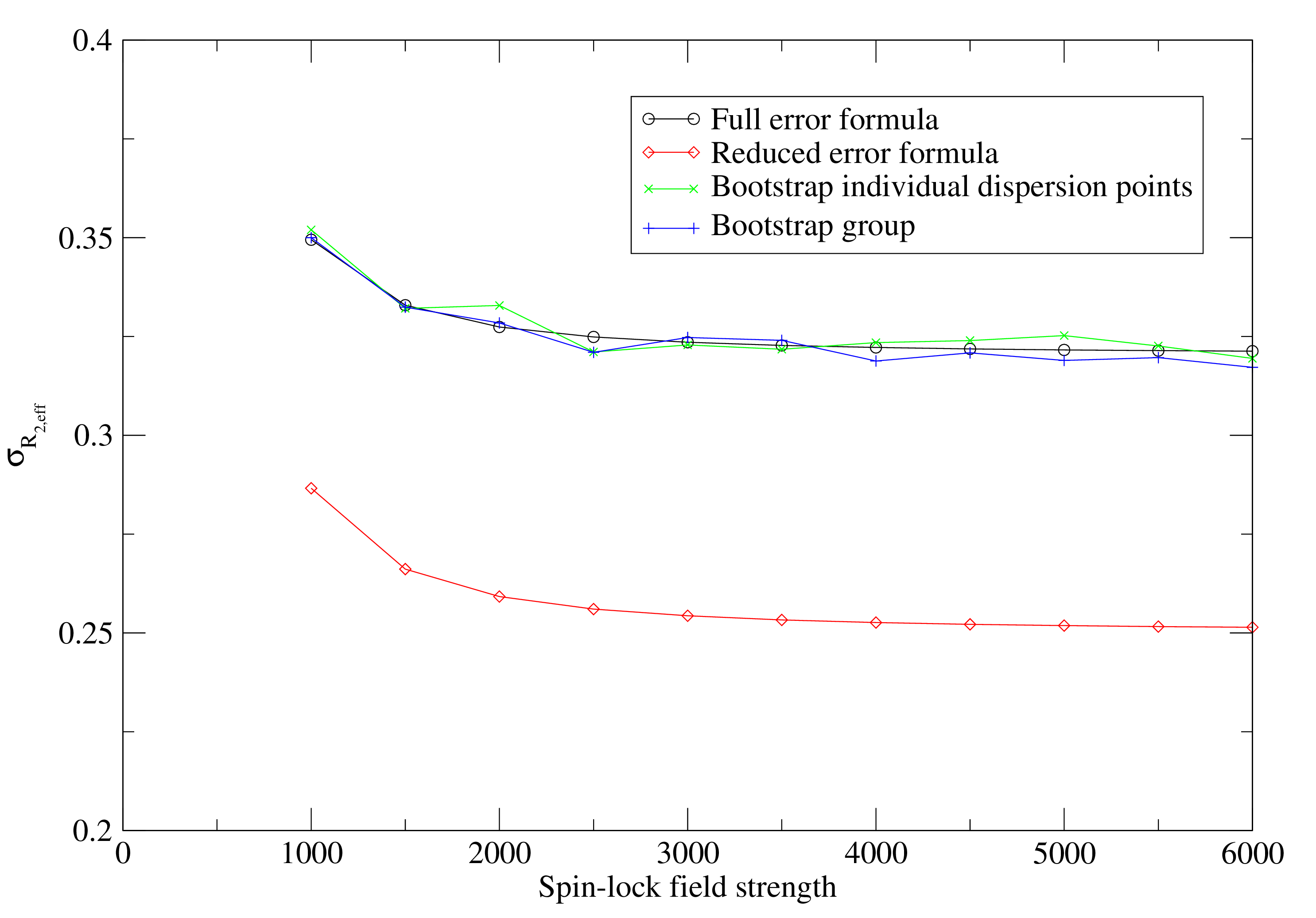
In a number of publications, the error formula from Ishima and Torchia (2005) has been used. This is the collapse of Equation 11.4 by setting σ_I₀ to zero:

This is not implemented in relax as it can be shown by simple simulation that the formula is incorrect (see Figure 11.1). This formula significantly underestimates the real errors. The use of the same I₀ value for all dispersion points does not cause a decrease in the R_2eff error but rather a correlation in the errors.

**Figure 11.1:** A demonstration of the inaccuracy of the error formula of Equation 11.12 from Ishima and Torchia (2005). This plot was generated using the script test_suite/shared_data/dispersion/error_testing/simulation.py. The bootstrapping simulation involves randomising noise-free I₀ and I₁ values for each dispersion data point assuming Gaussian errors. The full error formula is from Equation 11.4, the reduced error formula is from Equation 11.12, the bootstrapping using individual dispersion points estimates the errors assuming different I₀ randomisations for each dispersion point and each simulation, and the bootstrapping group graph uses the same randomised I₀ value for all dispersion points for each simulation.

Variable relaxation period experiments

For the variable relaxation time period type experiments, the R_2eff/ R_1ρ values are determined by fitting to the simple two parameter exponential as in a R₁ or R₂ analysis. Both R_2eff/ R_1ρ and the initial peak intensity I₀ are optimised using the minimise user function for each exponential curve separately. Monte Carlo simulations are used to obtain the parameter errors.

The R2eff model

Fixed relaxation period experiments

Variable relaxation period experiments

Links